
Paper
Form and function in hillslope hydrology: characterization of subsurface flow based on response observations
Abstract
The phrase form and function was established in architecture and biology and refers to the idea that form and functionality are closely correlated, influence each other, and co-evolve. We suggest transferring this idea to hydrologicalsystems to separate and analyze their two main characteristics: their form, which is equivalent to the spatial structure and static properties, and their function, equivalent to internal responses and hydrological behavior. While this approach is not particularly new to hydrological field research, we want to employ this concept to explicitly pursue the question of what information is most advantageous to understand a hydrological system. We applied this concept to subsurface flow within a hillslope, with a methodological focus on function: we conducted observations during a natural storm event and followed this with a hillslope-scale irrigation experiment. The results are used to infer hydrological processes of the monitored system. Based on these findings, the explanatory power and conclusiveness of the dataare discussed. The measurements included basic hydrological monitoring methods, like piezometers, soil moisture, and discharge measurements. These were accompanied by isotope sampling and a novel application of 2-D time-lapseGPR (ground-penetrating radar). The main finding regarding the processes in the hillslope was that preferential flowpaths were established quickly, despite unsaturated conditions. These flow paths also caused a detectable signal in the catchment response following a natural rainfall event, showing that these processes are relevant also at the catchment-scale. Thus, we conclude that response observations (dynamics and patterns, i.e., indicators of function) were well suited to describing processes at the observational scale. Especially the use of 2-D time-lapse GPR measurements, providing detailed subsurface response patterns, as well as the combination of stream-centered and hillslope-centered approaches,allowed us to link processes and put them in a larger context. Transfer to other scales beyond observational scale and generalizations, however, rely on the knowledge of structures (form) and remain speculative. The complementary approach with a methodological focus on form (i.e., structure exploration) is presented and discussed in the companion paper by Jackisch et al. (2017).
Figures from the paper
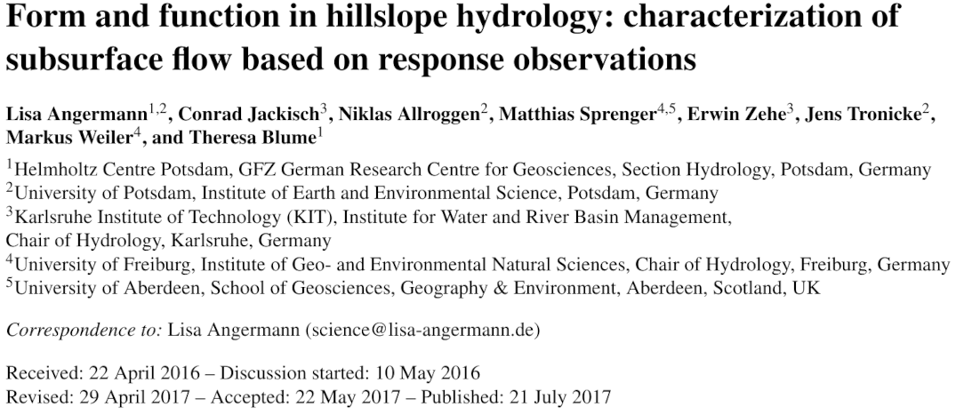
Figure 1
The concept of form and function applied to observations in hillslope hydrology. Four different categories which can be applied to data as well as the data sources.
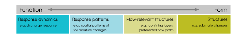
Figure 2
Map of the investigated Colpach River catchment and the four gauged sub-catchments. The site of the hillslope-scale irrigation experiment is located in the Holtz 2 catchment and is indicatedin red.
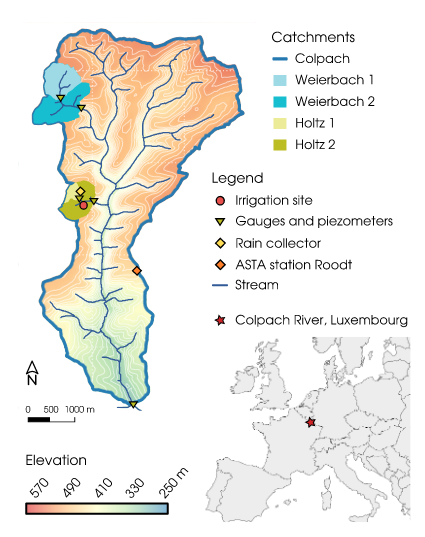
Figure 3
Experimental methods applied in the stream-centered and hillslope-centered approaches, divided into the sampling during the natural rain event and the irrigation experiment. Additionally, some structural background information was obtained from the literature and a digital elevation model.
Figure 4
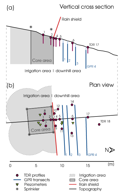
Vertical cross section (a) and plan view (b) of the experimental setup and sprinkler array. Location and depth of the TDR profiles and GPR ransects are given in purple and blue, respectively. The black line along the central TDR transect in (b) marks the vertical cross section depicted in (a).
Figure 5
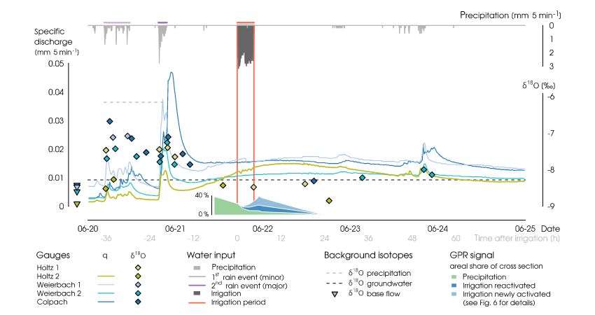
The figure shows the natural storm event on 20 June 2013 in the Colpach River catchment and the local intensity of the irrigationon 21 June 2013. The hydrographs below show the discharge response of four nested catchments (solid lines), in combination with the dynamics of the δ18O isotopic composition of the surface water (dots). The isotopic composition of the groundwater (annual mean) and the precipitation (daily values) are given by the dashed lines. Furthermore, the dynamic response of the GPR signal to natural and artificial rainfall is given in green and blue. While the first minor rain event caused only a weak response, the second event caused a double-peak discharge response in all sub-catchments. The irrigation experiment took place 19:22 h after the rain event
Figure 6
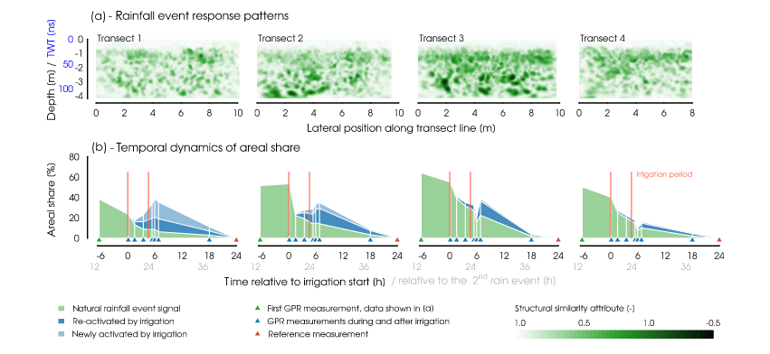
(a)Two-dimensional GPR data showing the subsurface response patterns caused by the natural rainfall event. The data show the structural similarity between the first GPR measurement (approximately 6:30 h before irrigation start and 12:52 h after the second rainfall event) and the last one. Low values of structural similarity are interpreted as high changes in soil moisture.
(b) Temporal dynamics of the areal share of active regions attributed to the natural rain event and the irrigation. Activated regions were identified by a structural similarity attribute of less than 0.85. Data were interpolated linearly between the measurements for visualization. The measurements shown in (a) show the data used to calculate the first data point shown in (b).
Figure 7
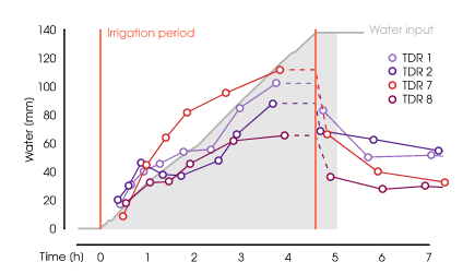
Water balance of the top 1.4 m of the soil column for the four core area TDR profiles. Dashed lines indicate the storage increase at the last measurement before irrigation ended. The variability between the four profiles shows the high heterogeneity and causes uncertainty regarding the average mass balance of the core area.
Figure 8
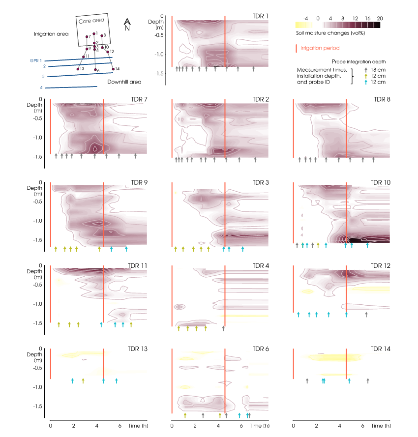
The soil moisture data measured at the TDR profiles at the irrigation site, showing the soil moisture dynamics in depth. The top four plots show all four core area profiles; columns are arranged according to the three diverging transects in the downhill direction. Rows are approximately at the same contour line. Measurements were taken at 0.1 m increments. While data analysis was based on non-interpolated data, soil moisture measurements were here interpolated linearly for better visualization. The plots cover the time from irrigation start until 9:00 h after irrigation start to focus on the first soil moisture response. Arrows indicate the measurement times and installation depth of eachTDR profile. Time is given in hours after irrigation start.
Figure 9
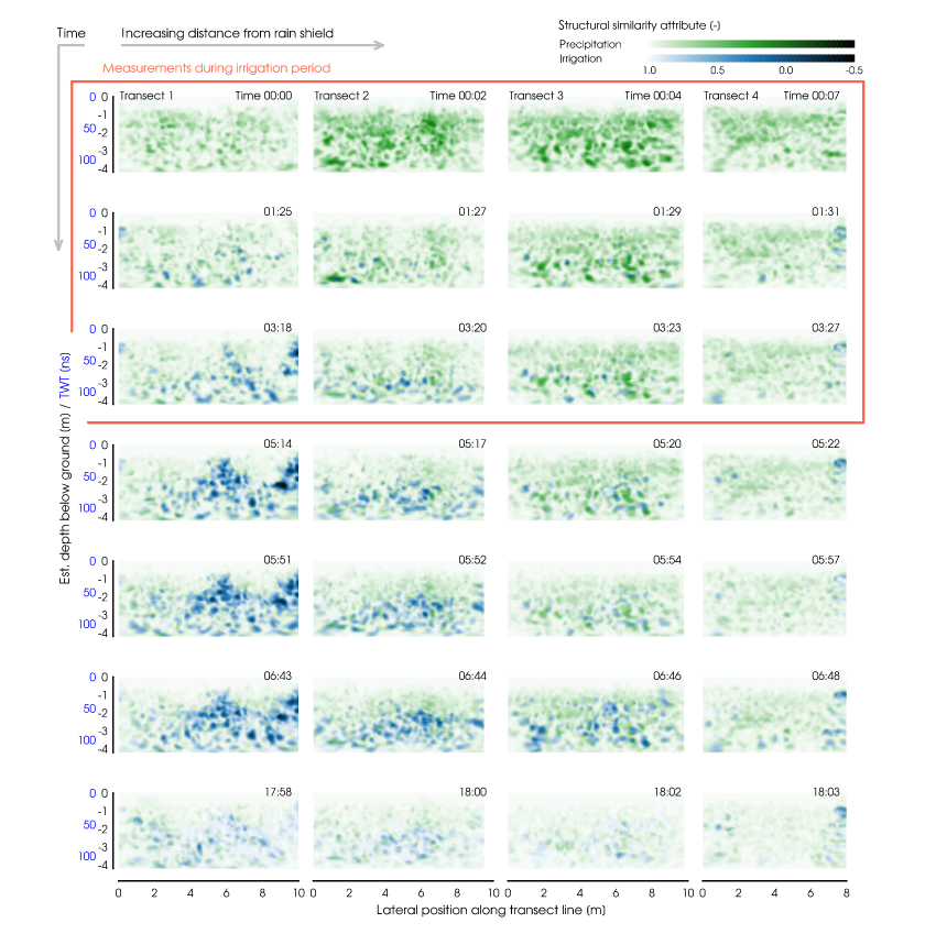
Structural similarity attributes calculated from time-lapse GPR data. All measurements were referenced to the last one 24:00 hafter irrigation start, indicating changes in the GPR reflection patterns associated with soil moisture changes. A structural similarity attribute value of 1 indicates full similarity; lower values signify higher deviation from the reference state. Water from the preceding natural rain event (green) was identified by constant or increasing structural similarity attributes. Water from the experimental irrigation (blue) was identifiedby decreasing values after irrigation start by more than 0.15. Within one column the rows give a sequence over time (after irrigation start). Columns proceed downhill, with increasing distance from the rain shield.
Figure 10
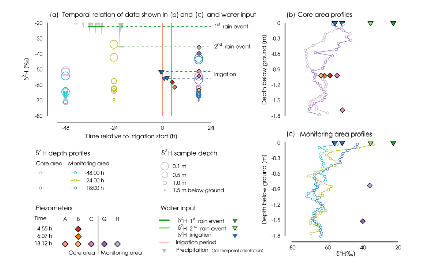
Stable isotope data from precipitation, irrigation, piezometers, and pore water samples.
(a) Temporal dynamics of pore water and piezometer δ2H in relation to water input by precipitation (bulk samples) and irrigation. Pore water data are shown only for the depths of piezometer filters (compare with panels (b) and (c) for depths) and the top soil (0.1 m below ground). The graph shows the direct impact of the water input (dashed lines) on the pore water isotope composition of the top soil.
(b, c) Pore water and piezometer data over depths, separated by core area and monitoring area. Water input stable isotope data are indicated at the soil surface
Figure 11
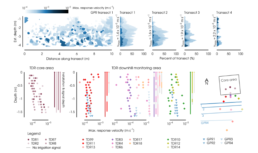
Top: depth distributions of response velocities calculated for the four time-lapse GPR transects. The blue scale indicates theresponse velocity calculated from the time of first arrival for each pixel. White areas did not show any irrigation water signal. The left plot shows the 2-D results for GPR transect 1. The margin plots on the right show the same data accumulated to 1-D depth profiles for all four GPR transects.
Bottom: response velocities calculated from TDR measurements at the core area (strictly vertical), and the downhill monitoring area (vertical and lateral). The three plots showing the TDR profiles at the downhill monitoring area are sorted according to the three diverging transects. Lines within the right margins of each TDR plot show the installation depths of the TDR profiles. Grey sections indicate depth increments that did not show a change in soil moisture. Additionally, GPR-based velocities derived from 0.5 m wide sections of the GPR transects close to the TDR profiles are shown.
Figure 12
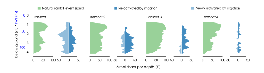
Areal share of activated regions per depth for the natural rainfall event and the irrigation. Areal share of activated regions forthe natural rain event were calculated from the first measurement only (also depicted in Fig. 6a). Values for the irrigation experiment were accumulated over all GPR measurements, counting every pixel that had been activated after irrigation start. Here, we distinguish between pixels that had been active before irrigation start and were re-activated again, and pixels which have not been active previously and were newly activated by irrigation.