Teaching material

During the years of the Corona pandemic, most teaching was conducted online. To make online lectures more vivid, I created short animations and a video tutorial series which lecturers at University of Potsdam used during their lessons.

Mathematical methods in geoecology

video tutorial series

For the lecture on mathematical methods in geoecology, I produced a series of short video tutorials to explain the application of certain mathematical methods for specific scientific questions. The topics and examples were chosen in collaboration with the lecturer and the style was set by former episodes of the format. The text, graphics, animation, sound recording, editing and postproduction was done by me.

The series featured the following episodes:

Introduction to the video tutorial series

Explaining the scientific workflow, introducing basic concepts and showcasing examples of applied mathematical methods in geoecology.

Differential equations

This episode shortly explains differential equations and uses them to predict the growth of a penguin population on an island, where exponential growth is limited by habitat capacity. This dynamics can mathematically be described by the logistic function, which is applied in many different contexts from ecology, to chemistry and economics.

Analyzing the diet of river trout populations

Based on calorimetric measurements of stomach content

Analysis of a tracer pulse injection experiment

Principle component analysis

Lecture script

Some of the examples from the video tutorial series were included in the lecture notes provided to students as a supplementary resource. I contributed texts and created figures that visualize the math behind the described examples and applications.

Flow velocity as derivative of the function of distance over time

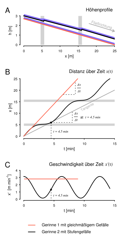
A: Höhenprofil zweier experimenteller Fließgerinne.
B: Entfernung des Tracerpulses vom Injektionspunkt über die Zeit.
C: Die erste Ableitung der Funktionen aus B zeigt die Veränderung der Fließgeschwindigkeit über die Zeit.

A: Elevation profile of two experimental flumes. B: Distance of the tracer pulse from the injection point over time. C: The first derivative of the functions in B shows the change in flow velocity over time.

Tracer mass as integral of the tracer concentration distribution

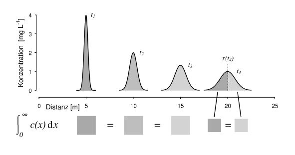
Tracerkonzentrationsverteilung entlang des Fließgerinnes zu verschiedenen Zeitpunkten t1, t2, t3 und t4. Während sich die Position und Form der Konzentrationsverteilung mit der Zeit ändern, bleibt die Fläche unter der Kurve konstant. Die Fläche unter der Kurve kann genutzt werden um den Schwerpunkt der Konzentrationsverteilung zu bestimmen

Tracer concentration distribution along the flume at different time points t1,t2,t3,t1​,t2​,t3​, and t4t4​. While the position and shape of the concentration distribution change over time, the area under the curve remains constant. This area can be used to determine the centroid of the concentration distribution.

Riemann Sum

The area under a curve can be approximated by dividing it into small rectangles. By summing the areas of these rectangles, we can estimate the total area below the curve. As the width of the rectangles approaches zero, their sum converges to the definite integral of the function, allowing us to calculate the exact area under the curve. This method is a fundamental concept in calculus and known as the Riemann Sum.

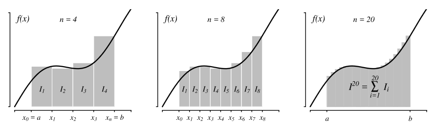
Verschiedene Näherungen des Integrals einer Funktion über einem Intervall [a, b] mit 4 (links), 8 (mittig) und 20 (rechts) Teilintervallen. Die Näherung konvergiert für “gutartige” (in diesem Falle zum Beispiel stetige) Funktionen gegen das tatsächliche Integral.

Various approximations of the integral of a function over the interval [a,b] using 4 (left), 8 (mid), and 20 (right) subintervals. The approximation converges to the actual integral for “well-behaved” functions (in this case a continuous function).

Vorlesungsskript “Mathematische Methoden in der Geoökologie”, Sabine Attinger, 2021

Feldmethoden in der Hydrologie

Principle of automated event-based sampling

This short animation was created for a lecture on hydrological field methods, to explain the setup and functioning of an automated event-based sampling device. The auto-sampler is connected to a gauge monitoring the water level of a stream. While the water level remains below a certain threshold, samples are taken at defined larger intervals to measure the background concentration. As soon as the water level exceeds the threshold, a shorter sampling interval is triggered to capture the dynamics during peak flow. After a defined amount of samples, the sampler returns to the background sampling intervall again.